Quick start

Short explanation on how to quickly run PAOS and have its output stored in a convenient file.

Running PAOS from terminal

The quickest way to run PAOS is from terminal.

Run it with the help flag to read the available options:

$ paos --help

The main command line flags are listed in Table 1.

Table 1 Main command line flags

flag	description
-h, --help	show this help message and exit
-c, --configuration	Input configuration file to pass
-o, --output	Output file
-p, --plot	Save output plots
-n, --nThreads	Number of threads for parallel processing
-d, --debug	Debug mode screen
-l, --logger	Store the log output on file

Where the configuration file shall be an .ini file and the output file an .h5 file (see later in The output file). -n must be followed by an integer. To activate -p, -d and -l no argument is needed.

Note

PAOS implements the log submodule which makes use of the python standard module logging for output information. Top-level details of the calculation are output at level logging.INFO, while details of the propagation through each optical plane and debugging messages are printed at level logging.DEBUG. The latter can be accessed by setting the flag -d, as explained above. Set the flag -l to redirect the logger output to a .log textfile.

Other option flags may be given to run specific simulations, as detailed in Table 2.

Table 2 Other option flags

flag	description
-wfe, --wfe_simulation	A list with wfe realization file and column to simulate an aberration

To have a lighter output please use the option flags listed in Table 3.

Table 3 Lighter output flags

flag	description
-keys, --keys_to_keep	A list with the output dictionary keys to save
-lo, --light_output	Save only at last optical surface

To activate -lo no argument is needed.

The output file

PAOS stores its main output product to a HDF5 file (extension is .h5 or .hdf5) such as that shown in Fig. 1. To open it, please choose your favourite viewer (e.g. HDFView, HDFCompass) or API (e.g. Cpp, FORTRAN and Python).

Fig. 1 Main PAOS output file

For more information on how to produce a similar output file, see Saving results.

The baseline plot

As part of the output, PAOS can plot the squared amplitude of the complex wavefront at a given point along the optical path (the focal plane in the case shown in Fig. 2).

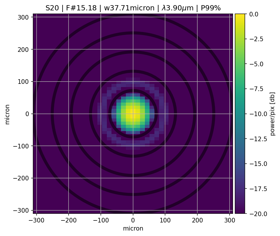
Fig. 2 Baseline PAOS plot

The title of the plot features the optical surface name, the focal number, the Gaussian beam width, the simulation wavelength and the total optical throughput that reaches the surface.

The color scale can be either linear or logarithmic. The x and y axes are in physical units, e.g. micron. For reference, black rings mark the first five zeros of the circular Airy function.

For more information on how to produce a similar plot, see Plotting results.