POP description
Brief description of some concepts of physical optics wavefront propagation (POP) and how they are implemented in PAOS, in the Fresnel approximation.
In PAOS, this is handled by the class WFO.
General diffraction
Diffraction is the deviation of a wave from the propagation that would be followed by a straight ray, which occurs when part of the wave is obstructed by the presence of a boundary. Light undergoes diffraction because of its wave nature.
The Huygens-Fresnel principle is often used to explain diffraction intuitively. Each point on the wavefront propagating from a single source can be though of as being the source of spherical secondary wavefronts (wavelets). The combination of all wavelets cancels except at the boundary, which is locally parallel to the initial wavefront.
However, if there is an object or aperture which obstructs some of the wavelets, changing their phase or amplitude, these wavelets interfere with the unobstructed wavelets, resulting in the diffraction of the wave.
Fresnel diffraction theory
Fresnel diffraction theory requires the following conditions to be met (see e.g. Lawrence et al., Applied Optics and Optical Engineering, Volume XI (1992)):
aperture sized significantly larger than the wavelength
modest numerical apertures
thin optical elements
PAOS is implemented assuming that Fresnel diffraction theory holds.
Coordinate breaks
Coordinate breaks are implemented as follows:
Decenter by \(x_{dec}, y_{dec}\)
Rotation XYZ (first X, then Y, then Z)
The rotation is intrinsic (X, then around new Y, then around new Z).
To transform the sagittal coordinates (\(x, u_{x}\)) and the tangential coordinates (\(y, u_{y}\)), define the position vector
and the unit vector of the light ray
where z is an appropriate projection of the unit vector such that \(u_{x}\) and \(u_{y}\) are the tangent of the angles (though we are in the paraxial approximation and this might not be necessary).
Note
z does not need to be calculated because it gets normalised away.
The position on the rotated \(x', y'\) plane would be \(\vec{R_0}'=(x', y', 0)\) and the relation is
that can be solved as
Example
Code example to use coordinate_break to simulate a coordinate break where the input
field is centered on the origin and has null angles \(u_{s}\) and \(u_{t}\) and is subsequently decentered on
the Y axis by \(y_{dec} = 10.0 \ \textrm{mm}\) and rotated around the X axis by \(x_{rot} = 0.1 ^{\circ}\).
import numpy as np
from paos.core.coordinateBreak import coordinate_break

field = {'us': 0.0, 'ut': 0.0}
vt = np.array([0.0, field['ut']])
vs = np.array([0.0, field['us']])

xdec, ydec = 0.0, 10.0e-3  # m
xrot, yrot, zrot = 0.1, 0.0, 0.0  # deg
vt, vs = coordinate_break(vt, vs, xdec, ydec, xrot, yrot, zrot, order=0.0)

print(vs, vt)
[0. 0.] [-0.01000002 0.00174533]
Gaussian beams
For a Gaussian beam, i.e. a beam with an irradiance profile that follows an ideal Gaussian distribution (see e.g. Smith, Modern Optical Engineering, Third Edition (2000))
where \(I_0\) is the beam intensity on axis, \(r\) is the radial distance and \(w\) is the radial distance at which the intensity falls to \(I_0 / e^2\), i.e., to 13.5 percent of its value on axis.
Note
\(w(z)\) is the semi-diameter of the beam and it encompasses \(86.5 \%\) of the beam power.
Due to diffraction, a Gaussian beam will converge and diverge from the beam waist \(w_0\), an area where the beam diameter reaches a minimum size, hence the dependence of \(w(z)\) on z, the longitudinal distance from the waist \(w_0\) to the plane of \(w(z)\), henceforward “distance to focus”.
A Gaussian beam spreads out as
where \(z_R\) is the Rayleigh distance.
A Gaussian beam is defined by just three parameters: \(w_0\), \(z_R\) and the divergence angle \(\theta\), as in Fig. 15 (from Edmund Optics, Gaussian beam propagation).

Fig. 15 Gaussian beam diagram
The complex amplitude of a Gaussian beam is of the form (see e.g. Lawrence et al., Applied Optics and Optical Engineering, Volume XI (1992))
where \(k\) is the wavenumber and \(R\) is the radius of the quadratic phase factor, henceforward “phase radius”. This reduces to
at the waist, where the wavefront is planar (\(R \rightarrow \infty\)).
Rayleigh distance
The Rayleigh distance of a Gaussian beam is defined as the value of z where the cross-sectional area of the beam is doubled. This occurs when w(z) has increased to \(\sqrt{2} w_0\).
Explicitly:
The physical significance of the Rayleigh distance is that it indicates the region where the curvature of the wavefront reaches a minimum value. Since
in the Rayleigh range, the phase radius is \(R = 2 z_R\).
From the point of view of the PAOS code implementation, the Rayleigh distance is used to develop a concept of near- and far-field,
to define specific propagators (see Wavefront propagation).
Gaussian beam propagation
To the accuracy of Fresnel diffraction, a Gaussian beam propagates as (see e.g. Lawrence et al., Applied Optics and Optical Engineering, Volume XI (1992))
where \(\theta(z)\) is a piston term referred to as the phase factor, given by
\(\theta(z)\) varies from \(\pi\) to \(-\pi\) when propagating from \(z = -\infty\) to \(z = \infty\).
The Gaussian beam propagation can also be described using ABCD matrix optics. A complex radius of curvature \(q(z)\) is defined as:
Propagating a Gaussian beam from some initial position (1) through an optical system (ABCD) to a final position (2) gives the following transformation:
Example
Code example to use WFO to estimate Gaussian beam properties for a given beam with diameter
\(d = 1.0\) m, before and after inserting a Paraxial lens with focal length \(f = 1.0\) m, and after
propagating to the lens focus. The zoom parameter is set to \(z = 4\).
Important
The zoom parameter is the ratio between the grid’s linear dimension and the beam size.
from paos.classes.wfo import WFO

beam_diameter = 1.0  # m
wavelength = 3.0e-6
grid_size = 512
zoom = 4

wfo = WFO(beam_diameter, wavelength, grid_size, zoom)

print('Pilot Gaussian beam properties\n')

print('Before lens\n')
print(f'Beam waist: {wfo.w0:.1e}')
print(f'Beam waist at current beam position: {wfo.wz:.1f}')
print(f'z-coordinate of the beam waist: {wfo.zw0:.1f}')
print(f'Rayleigh distance: {wfo.zr:.1e}')
print(f'Focal ratio: {wfo.fratio}')

fl = 1.0  # m
wfo.lens(lens_fl=fl)

print('\nAfter lens\n')
print(f'Beam waist: {wfo.w0:.1e}')
print(f'Beam waist at current beam position: {wfo.wz:.1f}')
print(f'z-coordinate of the beam waist: {wfo.zw0:.1f}')
print(f'Rayleigh distance: {wfo.zr:.1e}')
print(f'Focal ratio: {wfo.fratio:.1f}')

wfo.propagate(dz=fl)

print('\nAfter propagation to lens focus\n')
print(f'Beam waist: {wfo.w0:.1e}')
print(f'Beam waist at current beam position: {wfo.wz:.1e}')
print(f'z-coordinate of the beam waist: {wfo.zw0:.1f}')
print(f'Rayleigh distance: {wfo.zr:.1e}')
print(f'Focal ratio: {wfo.fratio:.1f}')
Pilot Gaussian beam properties

Before lens

Beam waist: 5.0e-01
Beam waist at current beam position: 0.5
z-coordinate of the beam waist: 0.0
Rayleigh distance: 2.6e+05
Focal ratio: inf

After lens

Beam waist: 1.9e-06
Beam waist at current beam position: 0.5
z-coordinate of the beam waist: 1.0
Rayleigh distance: 3.8e-06
Focal ratio: 1.0

After propagation to lens focus

Beam waist: 1.9e-06
Beam waist at current beam position: 1.9e-06
z-coordinate of the beam waist: 1.0
Rayleigh distance: 3.8e-06
Focal ratio: 1.0
Gaussian beam magnification
The Gaussian beam magnification can also be described using ABCD matrix optics. Using the definition given in Magnification, in this case
Therefore, for the complex radius of curvature we have that
Using the definition of \(q(z)\) it follows that
\(R_2 = M^2 R_1\)
\(w_2 = M w_1\)
for the phase radius and the semi-diameter of the beam, while from the definition of Rayleigh distance it follows that
\(z_{R,2} = M^2 z_{R,1}\)
\(w_{0,2} = M w_{0,1}\)
\(z_2 = M^2 z_1\)
for the Rayleigh distance, the Gaussian beam waist and the distance to focus.
Note
In the current version of PAOS, the Gaussian beam width is set along x. So, only the sagittal magnification changes
the Gaussian beam properties. A tangential magnification changes only the curvature of the
propagating wavefront.
Example
Code example to use WFO to simulate a magnification of the beam for the tangential direction
\(M_t = 3.0\), while keeping the sagittal direction unchanged (\(M_s = 1.0\)).
from paos.classes.wfo import WFO

beam_diameter = 1.0  # m
wavelength = 3.0e-6
grid_size = 512
zoom = 4

wfo = WFO(beam_diameter, wavelength, grid_size, zoom)

print('Before magnification\n')
print(f'Beam waist: {wfo.w0}')

Ms, Mt = 1.0, 3.0
wfo.Magnification(Ms, Mt)

print('\nAfter magnification\n')
print(f'Beam waist: {wfo.w0}')
Before magnification

Beam waist: 0.5

After magnification

Beam waist: 1.5
As a result, the semi-diameter of the beam increases three-fold.
Gaussian beam change of medium
As seen in Medium change, a change of medium from \(n_1\) to \(n_2\) can be described using an ABCD matrix with
Therefore, for the complex radius of curvature we have that
Using the definition of \(q(z)\) it follows that
\(R_2 = R_1 n_2/n_1\)
\(w_2 = w_1\)
\(z_{R,2} = z_{R,1} n_2/n_1\)
\(w_{0,2} = w_{0,1}\)
\(z_2 = z_1 n_2/n_1\)
For the phase radius, the semi-diameter of the beam, the Rayleigh distance, the Gaussian beam waist and the distance to focus, respectively.
Moreover, since \(\lambda_{2} = \lambda_{1} n_2/n_1\), it follows that
Example
Code example to use WFO to simulate a change of medium from \(n_1 = 1.0\) to \(n_2 = 1.5\),
to point out the change in distance to focus.
from paos.classes.wfo import WFO

beam_diameter = 1.0  # m
wavelength = 3.0e-6
grid_size = 512
zoom = 4

wfo = WFO(beam_diameter, wavelength, grid_size, zoom)
fl = 1.0  # m
wfo.lens(lens_fl=fl)

print('Before medium change\n')
print(f'Distance to focus: {wfo.distancetofocus:.1f}')

n1, n2 = 1.0, 1.5
wfo.ChangeMedium(n1n2=n1/n2)

print('\nAfter medium change\n')
print(f'Distance to focus: {wfo.distancetofocus:.1f}')
Before medium change

Distance to focus: 1.0

After medium change

Distance to focus: 1.5
Wavefront propagation
The methods for propagation are the hardest part of the problem of modelling the propagation through a
well-behaved optical system. A thorough discussion of this problem is presented in
Lawrence et al., Applied Optics and Optical Engineering, Volume XI (1992).
Here we discuss the relevant aspects for the PAOS code implementation.
Once an acceptable initial sampling condition is established and the propagation is initiated, the beam starts to spread due to diffraction. Therefore, to control the size of the array so that beam aliasing does not change much from the initial state it is important to choose the right propagator (far-field or near-field).
PAOS propagates the pilot Gaussian beam through all optical surfaces to calculate the beam width at all points in space.
The Gaussian beam acts as a surrogate of the actual beam and the Gaussian beam parameters inform the POP simulation.
In particular the Rayleigh distance \(z_R\) is used to inform the choice of specific propagators.
Aliasing occurs when the beam size becomes comparable to the array size. Instead of adjusting the sampling period to track exactly, it is more effective to have a region of constant sampling period near the beam waist (constant coordinates system of the form \(\Delta x_2 = \Delta x_1\)) and a linearly increasing sampling period far from the waist (expanding coordinates system of the form \(\Delta x_2 = \lambda |z|/M \Delta x_1\)).
For a given point, there are four possibilities in moving from inside or outside to inside or outside the Rayleigh range (RR), defined as the region between \(-z_R\) and \(z_R\) from the beam waist:
The situation is described in Fig. 16, taken from Lawrence et al., Applied Optics and Optical Engineering, Volume XI (1992).
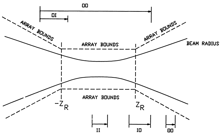
Fig. 16 Wavefront propagators
Explicitly, these possibilities are:
II(\(z_1\), \(z_2\)): inside RR to inside RR
IO(\(z_1\), \(z_2\)): inside RR to outside RR
OI(\(z_1\), \(z_2\)): outside RR to inside RR
OO(\(z_1\), \(z_2\)): outside RR to outside RR
To move from any point in space to any other, following Lawrence et al., Applied Optics and Optical Engineering, Volume XI (1992),
PAOS implements three primitive operators:
plane-to-plane (PTP): far-field
waist-to-spherical (WTS): far-field to near-field
spherical-to-waist (STW): near-field to far-field
Using these primitive operators, PAOS implements all possible propagations:
II(\(z_1\), \(z_2\)) = PTP(\(z_2-z_1\))
IO(\(z_1\), \(z_2\)) = WTS(\(z_2-z(w)\)) PTP(\(z(w)-z_1\))
OI(\(z_1\), \(z_2\)) = PTP(\(z_2-z(w)\)) STW(\(z(w)-z_1\))
OO(\(z_1\), \(z_2\)) = WTS(\(z_2-z(w)\)) STW(\(z(w)-z_1\))
Example
Code example to use WFO to propagate the beam over a thickness of \(10.0 \ \textrm{mm}\).
from paos.classes.wfo import WFO

wfo = WFO(beam_diameter, wavelength, grid_size, zoom)
print(f'Initial beam position: {wfo.z}')

thickness = 10.0e-3  # m
wfo.propagate(dz = thickness)
print(f'Final beam position: {wfo.z}')
Initial beam position: 0.0
Final beam position: 0.01
The current beam position along the z-axis is now updated.
Wavefront phase
A lens modifies the phase of an incoming beam.
Consider a monochromatic collimated beam travelling with slope \(u = 0\), incident on a paraxial lens, orthogonal to the direction of propagation of the beam. The planar beam is transformed into a converging or diverging beam. That means, a spherical wavefront with curvature \(>0\) for a converging beam, or a \(<0\) for a diverging beam.
The convergent beam situation is described in Fig. 17.

Fig. 17 Diagram for convergent beam
where:
the paraxial lens is coloured in red
the converging beam cone is coloured in blue
the incoming beam intersects the lens at a coordinate y
and
\(z\) is the propagation axis (\(>0\) at the right of the lens)
\(f\) is the optical focal length
\(\Delta z\) is the sag
\(\theta\) is the angle corresponding to the sag
\(\Delta z\) depends from the x and y coordinates, and it introduces a delay in the complex wavefront \(a_1(x, y, z) = e^{2\pi j z / \lambda}\) incident on the lens (\(z=0\) can be assumed). That is:
The sag can be estimated using the Pythagoras theorem and evaluated in small angle approximation, that is
The phase delay over the whole lens aperture is then
Sloped incoming beam
When the incoming collimated beam has a slope \(u_1\), its phase on the plane of the lens is given by \(e^{2\pi j y u_1 / \lambda}\) to which the lens adds a spherical sag.
This situation is described in Fig. 18.

Fig. 18 Diagram for convergent sloped beam
The total phase delay is then
Apart from the constant phase term, that can be neglected, this is a spherical wavefront centred in \((0, y_0, f)\), with \(y_0 = f u_1\).
Note
In this approximation, the focal plane is planar.
Off-axis incoming beam
The case of off-axis optics is described in Fig. 19.

Fig. 19 Diagram for off-axis beam
In this case, the beam centre is at \(y_c\).
Let \(\delta y\) be a displacement from \(y_c\) along y. The lens induced phase change is then
If the incoming beam has a slope \(u_1\), then
Apart from constant phase terms, that can be neglected, this is equivalent to a beam that is incident on-axis on the lens. The overall slope shifts the focal point in a planar focal plane. No aberrations are introduced.
Paraxial phase correction
For an optical element that can be modeled using its focal length \(f\) (that is, mirrors, thin lenses and refractive surfaces), the paraxial phase effect is
where t(x, y) is the complex transmission function. In other words, the element imposes a quadratic phase shift. The phase shift depends on initial and final position with respect to the Rayleigh range (see Wavefront propagation).
As usual, in PAOS this is informed by the Gaussian beam parameters. The code implementation consists of four
steps:
estimate the Gaussian beam curvature after the element (object space) using Eq. (27)
check the initial position using Eq. (37)
estimate the Gaussian beam curvature after the element (image space)
check the final position
By combining the result of the second and the fourth step, PAOS selects the propagator (see Wavefront propagation),
and the phase shift is imposed accordingly by defining a phase bias
(see Lawrence et al., Applied Optics and Optical Engineering, Volume XI (1992)):
Propagator |
Phase bias |
Description |
|---|---|---|
II |
\(1/f \rightarrow 1/f\) |
No phase bias |
IO |
\(1/f \rightarrow 1/f + 1/R'\) |
Phase bias after lens |
OI |
\(1/f \rightarrow 1/f - 1/R\) |
Phase bias before lens |
OO |
\(1/f \rightarrow 1/f - 1/R + 1/R'\) |
Phase bias before and after lens |
where \(R\) is the radius of curvature in object space and \(R'\) in image space.
Apertures
The actual wavefront propagated through an optical system intersects real optical elements (e.g. mirrors, lenses, slits) and can be obstructed by an object causing an obscuration.
For each one of these cases, PAOS implements an appropriate aperture mask. The aperture must be projected on the plane
orthogonal to the beam. If the aperture is (\(y_c, \phi_x, \phi_y\)), the aperture should be set as
Supported aperture shapes are elliptical, circular or rectangular.
Example
Code example to use WFO to simulate the beam propagation through an elliptical aperture with semi-major
axes \(x_{rad} = 0.55\) and \(y_{rad} = 0.365\), positioned at \(x_{dec} = 0.0\), \(y_{dec} = 0.0\).
from paos.classes.wfo import WFO

xrad = 0.55  # m
yrad = 0.365
xdec = ydec = 0.0

field = {'us': 0.0, 'ut': 0.1}
vt = np.array([0.0, field['ut']])
vs = np.array([0.0, field['us']])

xrad *= np.sqrt(1 / (vs[1] ** 2 + 1))
yrad *= np.sqrt(1 / (vt[1] ** 2 + 1))
xaper = xdec - vs[0]
yaper = ydec - vt[0]

wfo = WFO(beam_diameter, wavelength, grid_size, zoom)

aperture_shape = 'elliptical'  # or 'rectangular'
obscuration = False  # if True, applies obscuration

aperture = wfo.aperture(xaper, yaper, hx=xrad, hy=yrad,
                        shape=aperture_shape, obscuration=obscuration)

print(aperture)
Aperture: EllipticalAperture
positions: [256., 256.]
a: 70.4
b: 46.48813752661069
theta: 0.0
Stops
An aperture stop is an element of an optical system that determines how much light reaches the image plane. It is often the boundary of the primary mirror. An aperture stop has an important effect on the sizes of system aberrations.
The field stop limits the field of view of an optical instrument.
PAOS implements a generic stop normalizing the wavefront at the current position to unit energy.
Example
Code example to use WFO to simulate an aperture stop.
import numpy as np
from paos.classes.wfo import WFO

wfo = WFO(beam_diameter, wavelength, grid_size, zoom)

print('Before stop\n')
print(f'Total throughput: {np.sum(wfo.amplitude**2)}')

wfo.make_stop()

print('\nAfter stop\n')
print(f'Total throughput: {np.sum(wfo.amplitude**2)}')
Before stop

Total throughput: 262144.0

After stop

Total throughput: 1.0
POP propagation loop
PAOS implements the POP simulation through all elements of an optical system.
The simulation run is implemented in a single loop.
At first, PAOS initializes the beam at the centre of the aperture.
Then, it initializes the ABCD matrix.
Once the initialization is completed, PAOS repeats these actions in a loop:
Apply coordinate break
Apply aperture
Apply stop
Apply aberration (see Aberration)
Save wavefront properties
Apply magnification
Apply medium change
Apply lens
Apply propagation by thickness
Update ray vectors and ABCD matrices (and save them)
Repeat over all optical elements
Note
Each action is performed according to the configuration file, see Input system.
Example
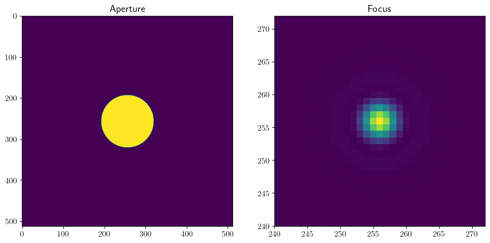
Code example to use WFO to simulate a simple propagation loop that involves key actions such as
applying a circular aperture, the throughput normalization, applying a Paraxial lens with focal length
\(f=1.0\) m, and propagating to the lens focus.
import matplotlib.pyplot as plt
from paos.classes.wfo import WFO

fig, (ax0, ax1) = plt.subplots(nrows=1, ncols=2, figsize=(12, 6))
wfo = WFO(beam_diameter, wavelength, grid_size, zoom)

wfo.aperture(xc=xdec, yc=ydec, r=beam_diameter/2, shape='circular')
wfo.make_stop()
ax0.imshow(wfo.amplitude**2)
ax0.set_title('Aperture')

fl = 1.0  # m
thickness = 1.0

wfo.lens(lens_fl=fl)
wfo.propagate(dz=thickness)
ax1.imshow(wfo.amplitude**2)
ax1.set_title('Focus')

zoomin = 16
shapex, shapey = wfo.amplitude.shape
ax1.set_xlim(shapex // 2 - shapex // 2 // zoomin, shapex // 2 + shapex // 2 // zoomin)
ax1.set_ylim(shapey // 2 - shapey // 2 // zoomin, shapey // 2 + shapey // 2 // zoomin)

plt.show()