Plotting results

PAOS implements different plotting routines, summarized here, that can be used to give a complementary idea of the main POP simulation results.

Base plot

The base plot method, simple_plot, receives as input the POP output dictionary and the dictionary key of one optical surface and plots the squared amplitude of the wavefront at the given optical surface.

Example

Code example to use simple_plot to plot the expected PSF at the image plane of the EXCITE optical chain.

import matplotlib.pyplot as plt
from paos.core.plot import simple_plot

fig = plt.figure(figsize=(8, 8))
ax = fig.add_subplot(1,1,1)

key = list(ret_val.keys())[-1]  # plot at last optical surface
simple_plot(fig, ax, key=key, item=ret_val[key], ima_scale='log')

plt.show()

The cross-sections for this PSF can be plotted using the method plot_psf_xsec, as shown below.

from paos.core.plot import plot_psf_xsec

fig = plt.figure(figsize=(9, 8))
ax = fig.add_subplot(1,1,1)

key = list(ret_val.keys())[-1]  # plot at last optical surface
plot_psf_xsec(fig, ax, key=key, item=ret_val[key], ima_scale='log')

plt.show()

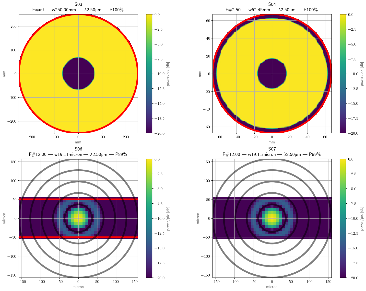
POP plot

The POP plot method, plot_pop, receives as input the POP output dictionary plots the squared amplitude of the wavefront at all available optical surfaces.

Example

Code example to use plot_pop to plot the squared amplitude of the wavefront at all surfaces of the EXCITE optical chain.

from paos.core.plot import plot_pop
plot_pop(ret_val, ima_scale='log', ncols=2)