Input system

PAOS has a generic input system to be used by anyone expert in Computer Aided Design (CAD).

Its two pillars are

1. The Configuration file

   A .ini configuration file with structure similar to that of Zemax OpticStudio \(^{©}\);

2. The GUI editor

   A GUI to dynamically modify the configuration file and launch instant POP simulations.

This structure allows the user to write configuration files from scratch or edit existing ones in a dynamic way, and to launch automatized POP simulations that reflect the edits without requiring advanced programming skills.

From a broad perspective, this input system has two advantages:

1. It can be used to design and test any optical system with relative ease.

   Outside Ariel, PAOS is currently used to simulate the optical performance of the stratospheric balloon-borne experiment EXCITE.

   Tip

   The interested reader may refer to the section Plot to see an example of PAOS results for EXCITE.

2. It helped in validating the PAOS code against existing simulators.

Configuration file

The configuration file is an .ini file structured into four different sections:

1. DEFAULT

   Optional section, not used

2. General

3. Wavelengths

4. Fields

5. Lens_xx

Note

PAOS defines units as follows:

1. Lens units: meters

2. Angles units: degrees

3. Wavelength units: micron

4. Temperature units: Celsius

5. Pressure units: atmospheres

General

Section describing the general simulation parameters and PAOS units

Table 4 General

keyword	type	description
project	string	A string defining the project name
version	string	Project version (e.g. 1.0)
grid_size	int	Grid size for simulation Must be in [64, 128, 512, 1024]
zoom	int	Zoom size Must be in [1, 2, 4, 8, 16]
lens_unit	string	Unit of lenses Must be ‘m’
tambient	float	Ambient temperature in Celsius
pambient	float	Ambient pressure in atmospheres

Below we report a snapshot of this section from the Ariel AIRS CH1 configuration file

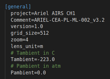
Fig. 3 General

Wavelengths

Section listing the wavelengths to simulate (preferably in increasing order)

Table 5 Wavelengths

keyword	type	description
w1	float	First wavelength
w2	float	Second wavelength
…	…	…

Below we report a snapshot of this section from the Ariel AIRS CH1 configuration file

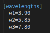
Fig. 4 Wavelengths

Fields

Section listing the input fields to simulate

Table 6 Fields

keyword	type	description
f1	float, float	Field 1: sagittal (x) and tangential (y) angle
f2	float, float	Field 2: sagittal (x) and tangential (y) angle
…	…	…

Below we report a snapshot of this section from the Ariel AIRS CH1 configuration file

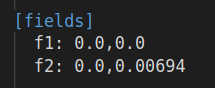
Fig. 5 Fields

Lens_xx

Lens data sections describing how to define the different optical surfaces (INIT, Coordinate Break, Standard, Paraxial Lens, ABCD, Zernike, PSD, and Grid Sag) and their required parameters.

Table 7 Lens_xx

SurfaceType	Comment	Radius	Thickness	Material	Save	Ignore	Stop	aperture	Par1..N
INIT	string, e.g. this surface name	None	None	None	None	None	None	list	None
Coordinate Break	…	None	float	None	Bool	Bool	Bool	None	None
Standard	…	float	float	MIRROR, others	Bool	Bool	Bool	list	None
Paraxial Lens	…	None	float	None	Bool	Bool	Bool	list	Par1 = focal length (float)
ABCD	…	None	float	None	Bool	Bool	Bool	list	Par1..4 = Ax, Bx, Cx, Dx (sagittal) Par5..8 = Ay, By, Cy, Dy (tangential)
Zernike In addition to standard parameters defines: Zindex: polynomial index starting from 0 Z: coefficients in units of wave	…	None	None	None	Bool	Bool	Bool	None or list	Par1 = wavelength (in micron) Par2 = ordering, can be standard, ansi, noll, fringe Par3 = Normalisation, can be True or False Par4 = Radius of support aperture of the polynomial Par5 = origin, can be x (counterclockwise positive from x axis) or y (clockwise positive from y axis) Par6 = Zorthonorm, False (Zernike circular polynomials) or True (polynomials that are ortho-normal on the aperture provided)
PSD	…	None	None	None	Bool	Bool	Bool	None	Par1 = A Par2 = B Par3 = C Par4 = fknee Par5 = fmin Par6 = fmax Par7 = Surface Roughness Par8 = units (usually nm)
Grid Sag	…	None	None	None	Bool	Bool	Bool	None	Par1 = wavelength (in micron) Par2 = Nx (in pixel) Par3 = Ny (in pixel) Par4 = Dx Par5 = Dy Par6 = Xdecenter (in pixel) Par7 = Ydecenter (in pixel) Par8 = Errormap file path

Note

1. Set the Ignore flag to True to skip the surface

2. Set the Stop flag to True to make the surface a Stop (see Stops)

3. Set the Save flat to True to later save the output for the surface

Note

The aperture keyword is a list with the following format:

• aperture = shape type, wx, wy, xc, yc

• shape: either ‘elliptical’ or ‘rectangular’

• type: either ‘aperture’ or ‘obscuration’

• wx, wy: semi-axis of elliptical shapes, or full length of rectangular shape sides

• xc, yc: coordinates of aperture centre

Example: aperture = elliptical aperture, 0.5, 0.3, 0.0, 0.0

Note

The functional form of the PSD is given by:

\(PSD(f) = \frac{A}{B + (f/f_{knee})^C}\)

Below we report a snapshot of the first lens data section from the Ariel AIRS CH1 configuration file

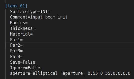
Fig. 6 Lens_xx

Parse configuration file

PAOS implements the method parse_config that parses the .ini configuration file, prepares the simulation run and returns the simulation parameters and the optical chain. This method can be called as in the example below.

Example

Code example to parse a PAOS configuration file.

from paos.core.parseConfig import parse_config
pup_diameter, parameters, wavelengths, fields, opt_chains = parse_config('path/to/ini/file')

GUI editor

PAOS implements a GUI editor that allows to dynamically edit and modify the configuration file and to launch POP simulations. This makes it effectively the PAOS front-end. To achieve this, PAOS (v1.2.1 and above) uses the shiny package, a Python package that supports the development of Python web applications with the power of reactive programming.

Note

Previous PAOS versions relied on the PySimpleGui package, however this has been discontinued due to a change in their policy.

The quickest way to run the PAOS GUI is from terminal.

Run it with the help flag to read the available options:

$ paos_gui --help

Table 8 GUI command line flags

flag	description
-h, --help	show this help message and exit
-d, --debug	Run the Shiny app in debug (auto-reload) mode.

Where the configuration file shall be an .ini file (see Configuration file).

The GUI editor then opens and displays a window with a standard File Menu (Open, Save, Close) and a Help Menu (Docs, About). The GUI has four Tabs:

1. System Explorer

2. Lens Editor

3. Wavefront Editor

4. Optical Analysis

The user can choose to work in dark mode using the switch on the right of the logo.

System Explorer

This Tab opens upon starting the GUI. Its purpose is to setup the main simulation parameters. It contains a sidebar, which displays the general simulation parameters and PAOS units, as defined in General. The contents can be altered as necessary, safe if the the cells are disabled. On the main tab area the wavelengths and fields are listed, as parsed from the configuration file.

Below we report a snapshot of this Tab.

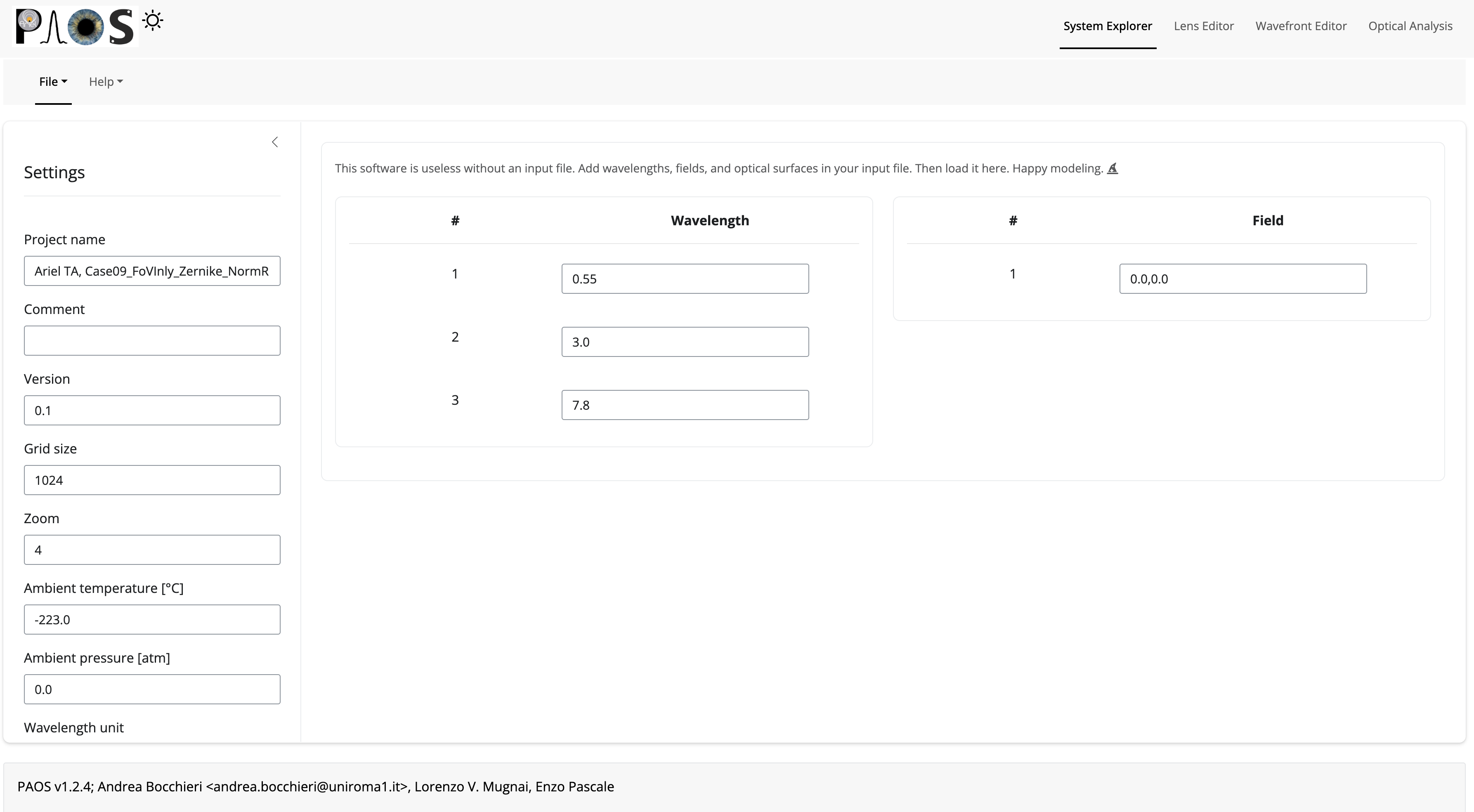
Fig. 7 System Explorer

Tip

You cannot add new wavelengths or fields in the GUI. This needs to happen in the configuration file. So, save your current work to a new .ini config file using File/Save and make any changes there. Then, reload the file to the GUI.

Lens Editor

This Tab contains the list of the optical surfaces describing the optical chain to simulate, as defined in Lens_xx.

This information is organized as explained in Lens_xx, with horizontal and vertical scrollbars to allow any movement.

The contents of each cell can be edited as necessary.

Tip

You cannot add new surfaces or change the surface type in the GUI. This needs to happen in the configuration file. So, save your current work to a new .ini config file using File/Save and make any changes there. Then, reload the file to the GUI.

Below we report a snapshot of this Tab.

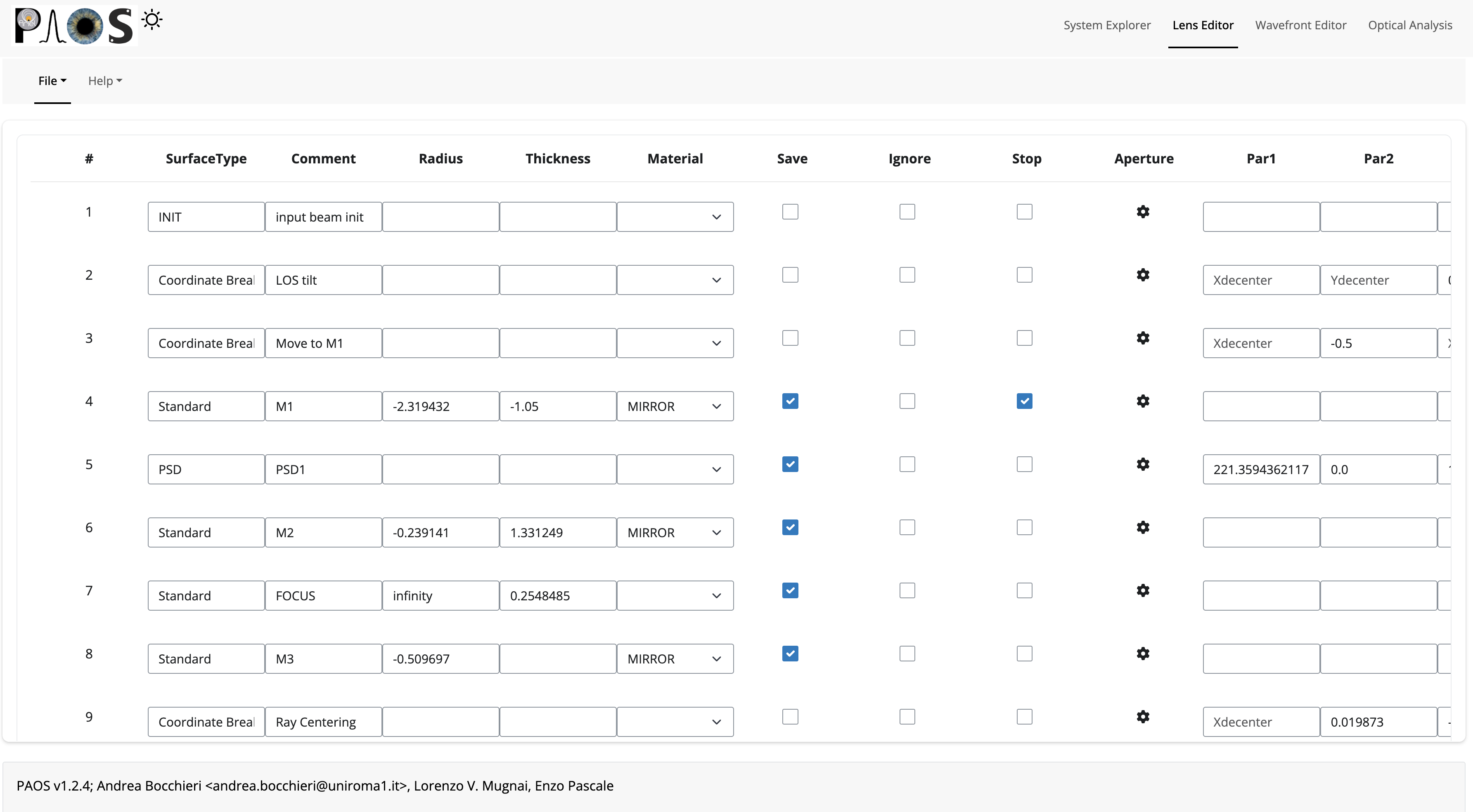
Fig. 8 Lens Editor

Tip

Placeholders in unused Par1..N parameter cells help remember the cell intended content.

Tip

To see/edit the contents of the Aperture column, click on the gear icon.

Wavefront Editor

This Tab contains three panels, each containing a sidebar as well as an Explorer and a Plot area. The sidebar allows the user to select the desired surface for modification or plotting.

• Zernike

  The Explorer area contains a Table that lists the Zernike (or ortho-normal) polynomial radial (n) and azimuthal (m) orders according to the specified Zernike ordering (one of standard, ansi, fringe and noll), the index as given by the user (Zindex), and the Zernike coefficients (Z). Only the Z column is enabled to be modified as required by the user. The Plot area allows the user to draw the aberrated surface that corresponds to the Zernike expansion in the table and save it to a file.

Below we report a snapshot of this panel.

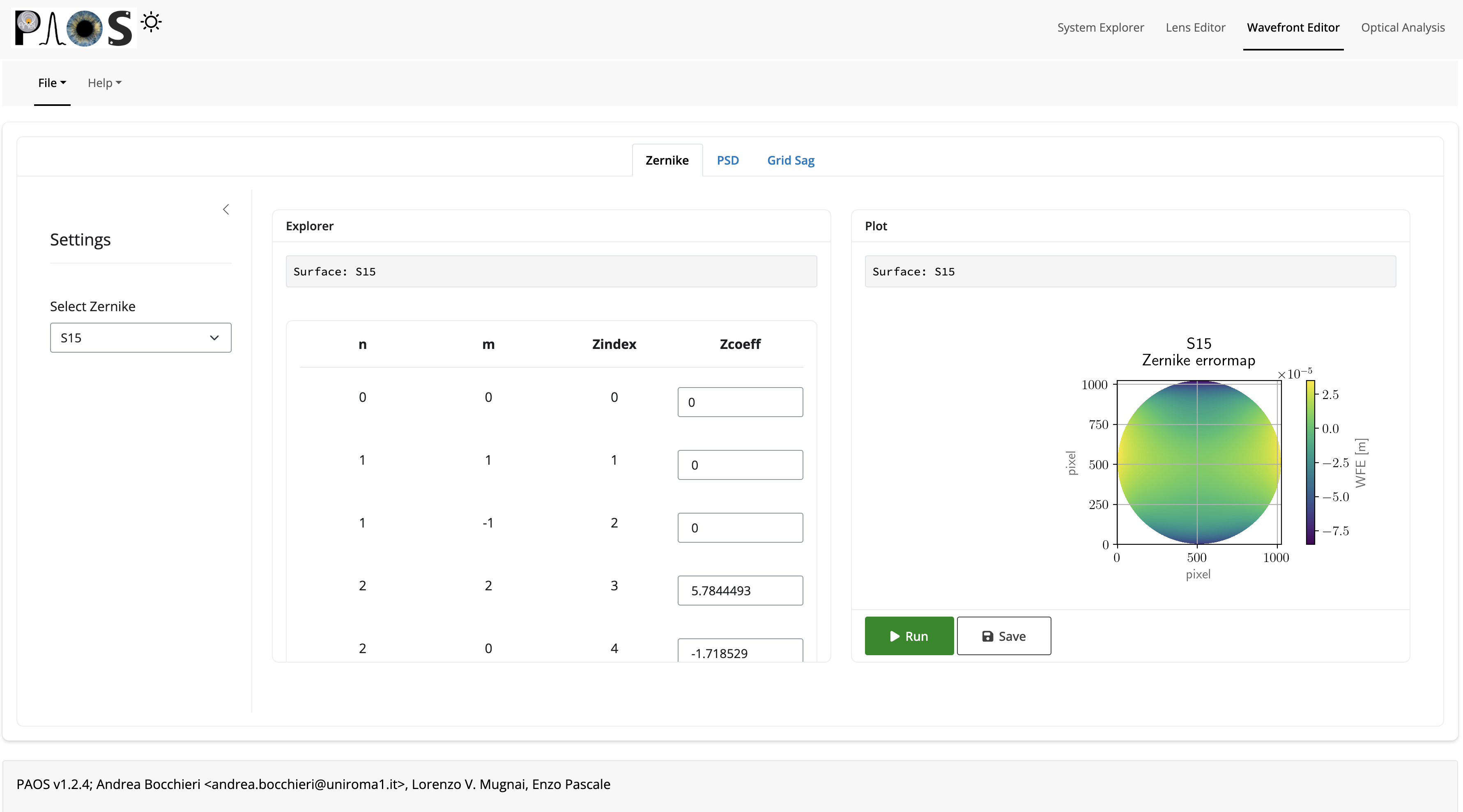
Fig. 9 Zernike Panel

• PSD

  The Explorer area contains a calculator for the Surface Form Error that corresponds to the PSD parameters (and Surface Roughness), input by the user in the Lens Editor. The Plot area allows one to draw the aberrated surface that corresponds to the PSD and save it to a file. The gear icon on the Plot header allows one to change the spatial scale for the plot. E.g. the user can draw the PSD on a 1 mm-diameter circle rather than 1-m to better visualize local deformations.

Below we report a snapshot of this panel.

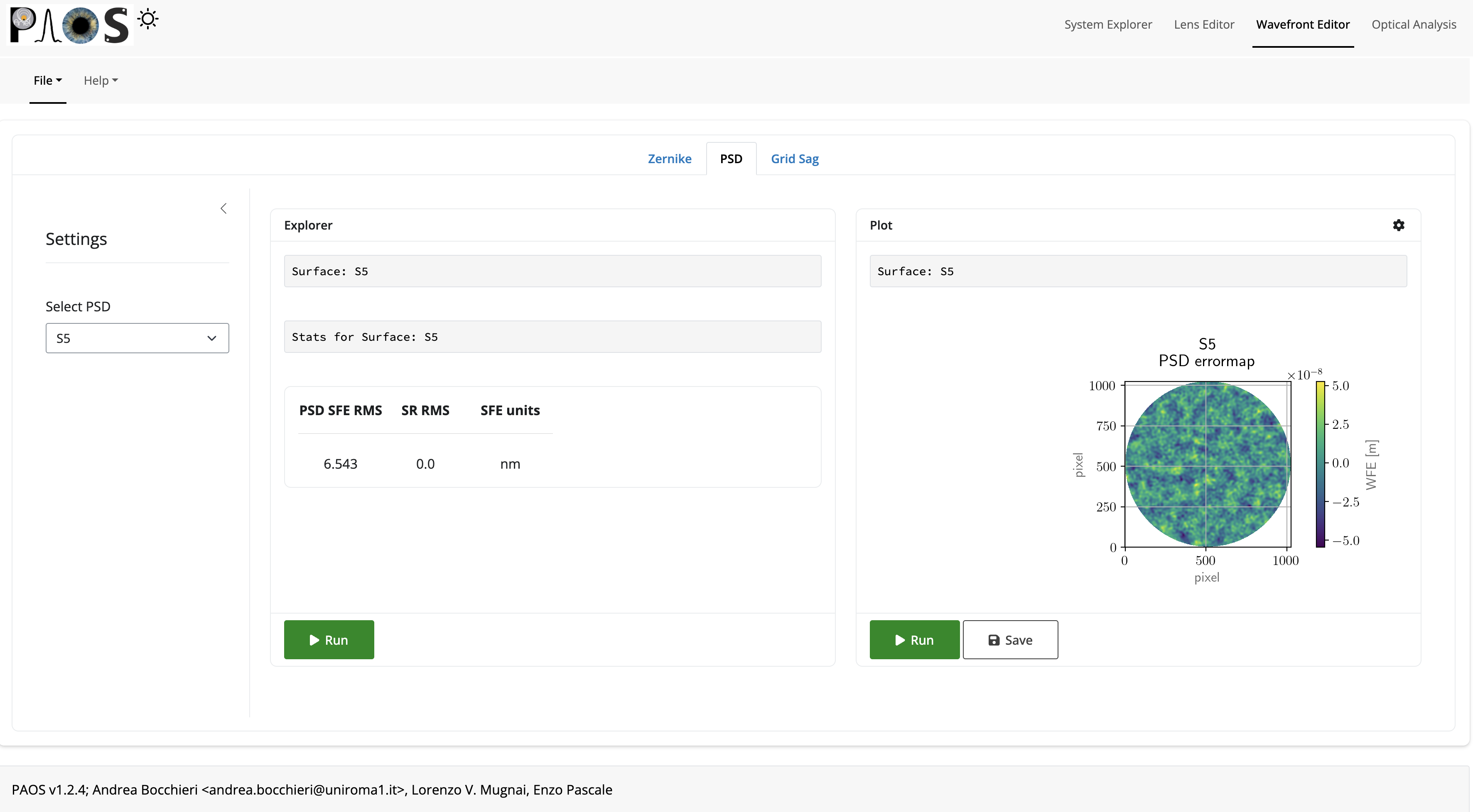
Fig. 10 PSD Panel

• Grid Sag

  The Explorer area only contains an output text that reports the file path of the errormap input by the user in the Lens Editor. The Plot area allows one to draw the aberrated surface that corresponds to the input Grid Sag and save it to a file.

Below we report a snapshot of this panel.

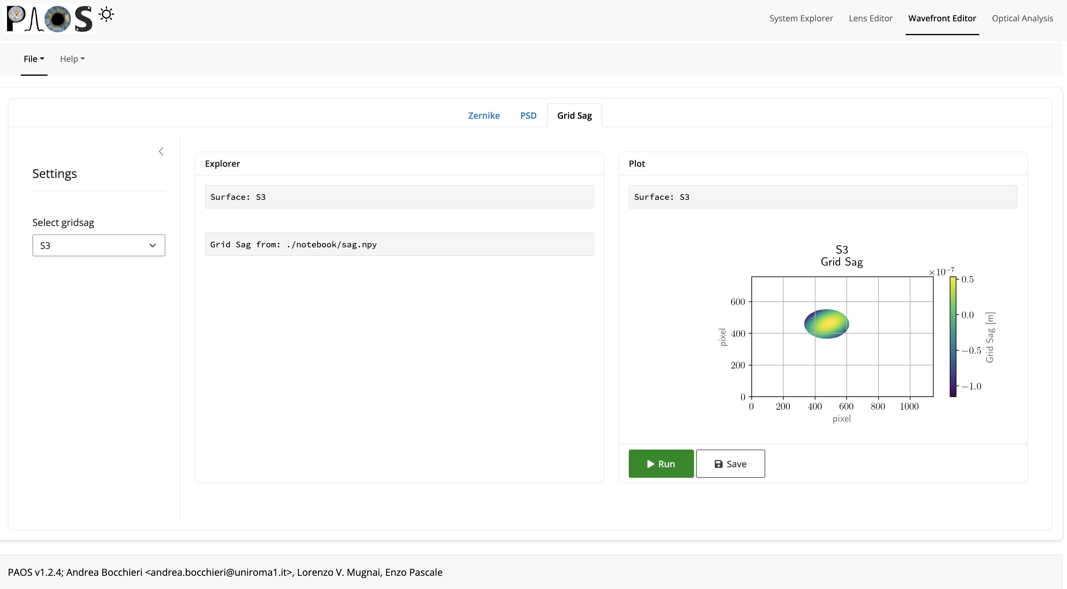
Fig. 11 Grid Sag Panel

Optical Analysis

This Tab provides the main GUI functionality: the POP propagation. It is updated dinamically based on the parameters input by the user in the System Explorer, Lens Editor, and Wavefront Editor tabs. The POP simulation is done one wavelength and field at a time, which can be chosen from the dropdown menus in the sidebar.

The main part of the Tab contains three panels:

• Fresnel POP

  Allows to run the wavefront propagation simulation and save the outputs to a binary (.hdf5) file.

• Ray Tracing

  Allows to run user to a diagnostic ray-trace of the optical system, producing an output that is displayed in the text area and can be saved to a text file.

• Plot

  Allows one to draw the squared amplitude of the wavefront. The gear icon on the Plot header contains options for selecting a different surface (any surface with Save = True in the Lens_xx), changing the plot scale (linear or log), zoom factor (the greater, the more zoomed out), and an option to plot dark rings in correspondance to the first 5 zeros of the Airy diffraction pattern. The plot can then be saved to a (.pdf) or (.png) file.

Below we report a snapshot of this Tab.

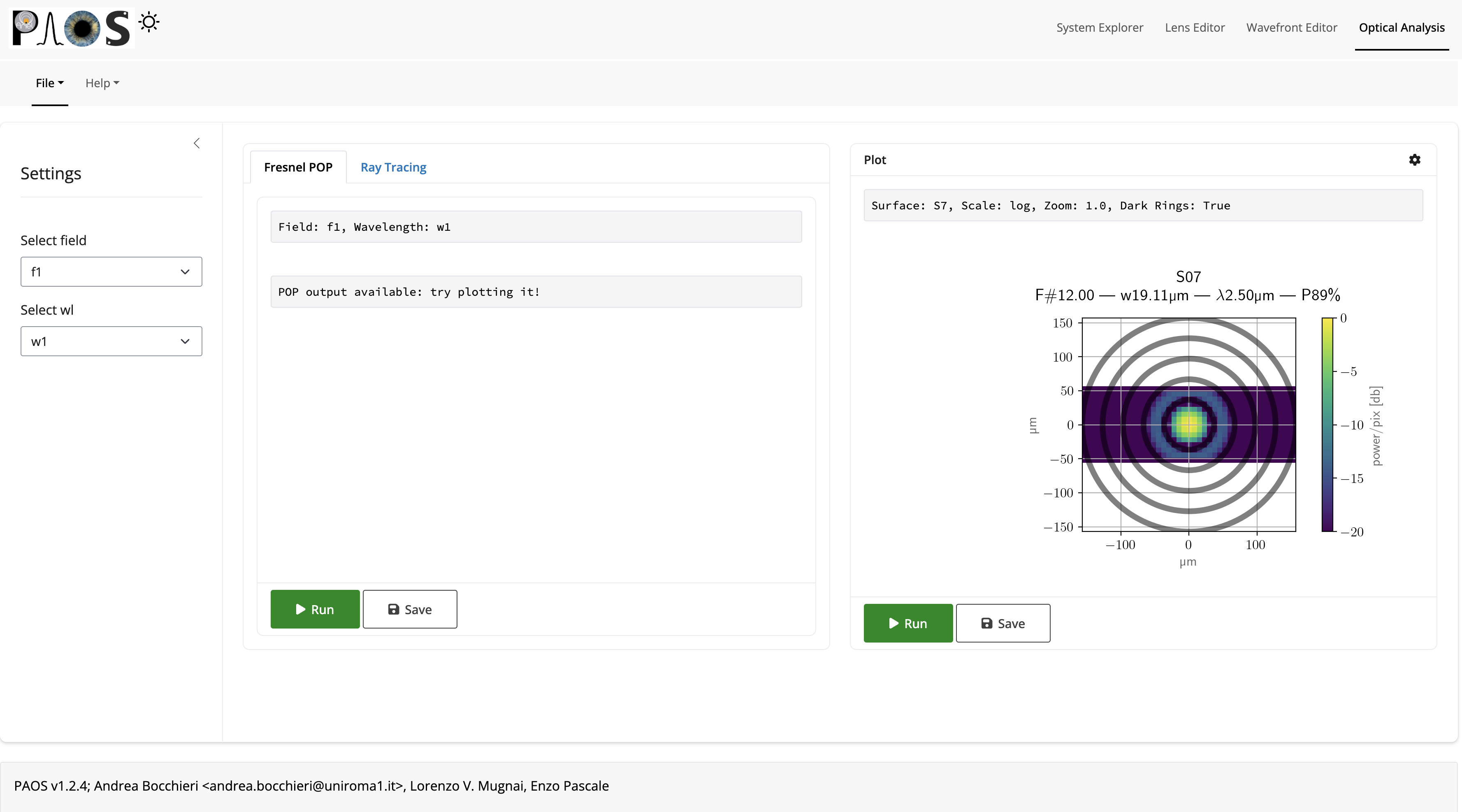
Fig. 12 Optical Analysis Tab